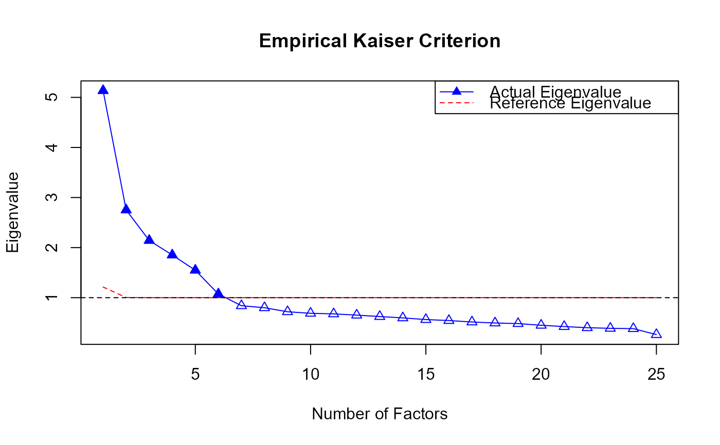
Empirical Kaiser Criterion — EKC • EFAfactors

This function will apply the Empirical Kaiser Criterion (Braeken & van Assen, 2017) method to determine the number of factors. The method assumes that the distribution of eigenvalues asymptotically follows a Marcenko-Pastur distribution (Marcenko & Pastur, 1967). It calculates the reference eigenvalues based on this distribution and determines whether to retain a factor by comparing the size of the empirical eigenvalues to the reference eigenvalues.

EKC(
  response,
  cor.type = "pearson",
  use = "pairwise.complete.obs",
  vis = TRUE,
  plot = TRUE
)

Arguments

response: A required N × I matrix or data.frame consisting of the responses of N individuals to I items.
cor.type: A character string indicating which correlation coefficient (or covariance) is to be computed. One of "pearson" (default), "kendall", or "spearman". @seealso cor.
use: An optional character string giving a method for computing covariances in the presence of missing values. This must be one of the strings "everything", "all.obs", "complete.obs", "na.or.complete", or "pairwise.complete.obs" (default). @seealso cor.
vis: A Boolean variable that will print the factor retention results when set to TRUE, and will not print when set to FALSE. (default = TRUE)
plot: A Boolean variable that will print the EKC plot when set to TRUE, and will not print it when set to FALSE. @seealso plot.EKC. (Default = TRUE)

Value

An object of class EKC is a list containing the following components:

nfact: The number of factors to be retained.
eigen.value: A vector containing the empirical eigenvalues
eigen.ref: A vector containing the reference eigenvalues

Details

The Empirical Kaiser Criterion (EKC; Auerswald & Moshagen, 2019; Braeken & van Assen, 2017) refines Kaiser-Guttman Criterion by accounting for random sample variations in eigenvalues. At the population level, the EKC is equivalent to the original Kaiser-Guttman Criterion, extracting all factors whose eigenvalues from the correlation matrix are greater than one. However, at the sample level, it adjusts for the distribution of eigenvalues in normally distributed data. Under the null model, the eigenvalue distribution follows the Marčenko-Pastur distribution (Marčenko & Pastur, 1967) asymptotically. The upper bound of this distribution serves as the reference eigenvalue for the first eigenvalue $\lambda$, so

$$\lambda_{1,ref} = \left( 1 + \sqrt{\frac{I}{N}} \right)^2$$

, which is determined by N individuals and I items. For subsequent eigenvalues, adjustments are made based on the variance explained by previous factors. The j-th reference eigenvalue is:

$$\lambda_{j,ref} = \max \left[ \frac{I - \sum_{i=0}^{j-1} \lambda_i}{I - j + 1} \left( 1 + \sqrt{\frac{I}{N}} \right)^2, 1 \right]$$

The j-th reference eigenvalue is reduced according to the magnitude of earlier eigenvalues since higher previous values mean less unexplained variance remains. As in the original Kaiser-Guttman Criterion, the reference eigenvalue cannot drop below one.

$$F = \sum_{i=1}^{I} I(\lambda_i > \lambda_{i,ref})$$

Here, $ F $ represents the number of factors determined by the EKC, and $I(\cdot)$ is the indicator function, which equals 1 when the condition is true, and 0 otherwise.

References

Auerswald, M., & Moshagen, M. (2019). How to determine the number of factors to retain in exploratory factor analysis: A comparison of extraction methods under realistic conditions. Psychological methods, 24(4), 468-491. https://doi.org/10.1037/met0000200.

Braeken, J., & van Assen, M. A. L. M. (2017). An empirical Kaiser criterion. Psychological methods, 22(3), 450-466. https://doi.org/10.1037/met0000074.

Marcˇenko, V. A., & Pastur, L. A. (1967). Distribution of eigenvalues for some sets of random matrices. Mathematics of the USSR-Sbornik, 1, 457–483. http://dx.doi.org/10.1070/SM1967v001n04ABEH001994

Author

Haijiang Qin <Haijiang133@outlook.com>

Examples

library(EFAfactors)
set.seed(123)

##Take the data.bfi dataset as an example.
data(data.bfi)

response <- as.matrix(data.bfi[, 1:25]) ## loading data
response <- na.omit(response) ## Remove samples with NA/missing values

## Transform the scores of reverse-scored items to normal scoring
response[, c(1, 9, 10, 11, 12, 22, 25)] <- 6 - response[, c(1, 9, 10, 11, 12, 22, 25)] + 1


## Run EKC function with default parameters.
# \donttest{
 EKC.obj <- EKC(response)
#> The number of factors suggested by EKC is 6 .

 print(EKC.obj)
#> The number of factors suggested by EKC is 6 .

 plot(EKC.obj)


 ## Get the eigen.value, eigen.ref and  nfact results.
 eigen.value <- EKC.obj$eigen.value
 eigen.ref <- EKC.obj$eigen.ref
 nfact <- EKC.obj$nfact

 print(eigen.value)
#>  [1] 5.1343112 2.7518867 2.1427020 1.8523276 1.5481628 1.0735825 0.8395389
#>  [8] 0.7992062 0.7189892 0.6880888 0.6763734 0.6517998 0.6232530 0.5965628
#> [15] 0.5630908 0.5433053 0.5145175 0.4945031 0.4826395 0.4489210 0.4233661
#> [22] 0.4006715 0.3878045 0.3818568 0.2625390
 print(eigen.ref)
#>  [1] 1.212873 1.003940 1.000000 1.000000 1.000000 1.000000 1.000000 1.000000
#>  [9] 1.000000 1.000000 1.000000 1.000000 1.000000 1.000000 1.000000 1.000000
#> [17] 1.000000 1.000000 1.000000 1.000000 1.000000 1.000000 1.000000 1.000000
#> [25] 1.000000
 print(nfact)
#> [1] 6

# }