K-means for EFA

A function performs K-means algorithm on items by calling kmeans.

EFAkmeans(response, nfact.max = 10, plot = TRUE)

Arguments

response

A required N × I matrix or data.frame consisting of the responses of N individuals to I items.

nfact.max

The maximum number of factors discussed by EFAkmeans approach. (default = 10)

plot

A Boolean variable that will print the EFAkmeans plot when set to TRUE, and will not print it when set to FALSE. @seealso plot.EFAkmeans. (Default = TRUE)

Value

An object of class EFAkmeans is a list containing the following components:

wss

A vector containing all within-cluster sum of squares (WSS).

nfact.SOD

The number of factors to be retained by the Second-Order Difference (SOD) approach.

Details

K-means is a well-established and widely used classical clustering algorithm. It is an unsupervised machine learning algorithm that requires the number of clusters K to be specified in advance. After K-means terminates, the total within-cluster sum of squares (WSS) can be calculated to represent the goodness of fit of the clustering: $$WSS = \sum_{\mathbf{C}_k \in \mathbf{C}} \sum_{i \in \mathbf{C}_k} \|i - \mu_k\|^2$$

where \(\mathbf{C}\) is the set of all clusters. \(\mathbf{C}_k\) is the k-th cluster. \(i\) represents each item in the cluster \(\mathbf{C}_k\). \(\mu_k\) is the centroid of cluster \(\mathbf{C}_k\).

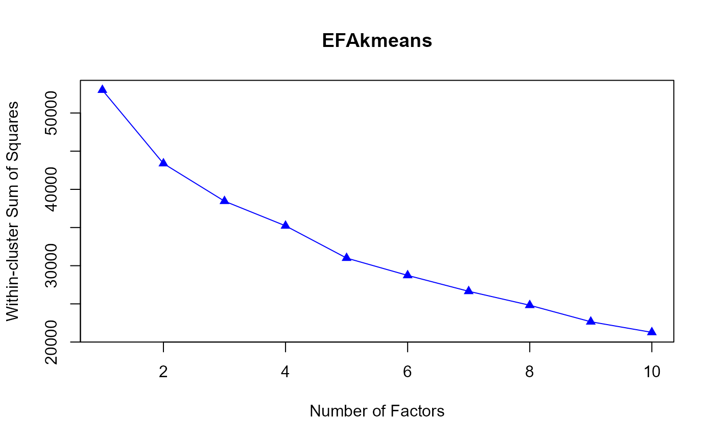
Similar to the scree plot where eigenvalues decrease as the number of factors increases, WSS also decreases as K increases. A "significant reduction" in WSS at a particular K may suggest that K is the most appropriate number of clusters, which in exploratory factor analysis implies that the number of factors is K. The "significant reduction" can be identified using the Second-Order Difference (SOD) approach. @seealso EFAkmeans

Examples

library(EFAfactors)
set.seed(123)

##Take the data.bfi dataset as an example.
data(data.bfi)

response <- as.matrix(data.bfi[, 1:25]) ## loading data
response <- na.omit(response) ## Remove samples with NA/missing values

## Transform the scores of reverse-scored items to normal scoring
response[, c(1, 9, 10, 11, 12, 22, 25)] <- 6 - response[, c(1, 9, 10, 11, 12, 22, 25)] + 1


## Run EFAkmeans function with default parameters.
# \donttest{
 EFAkmeans.obj <- EFAkmeans(response)

 plot(EFAkmeans.obj)


 ## Get the heights.
 wss <- EFAkmeans.obj$wss
 print(wss)
#>  [1] 53008.61 43385.54 38452.58 35222.24 30999.38 28729.83 26647.84 24820.24
#>  [9] 22657.66 21269.12

 ## Get the nfact retained by SOD
 nfact.SOD <- EFAkmeans.obj$nfact.SOD
 print(nfact.SOD)
#> [1] 2


# }